Population of London

Original Image

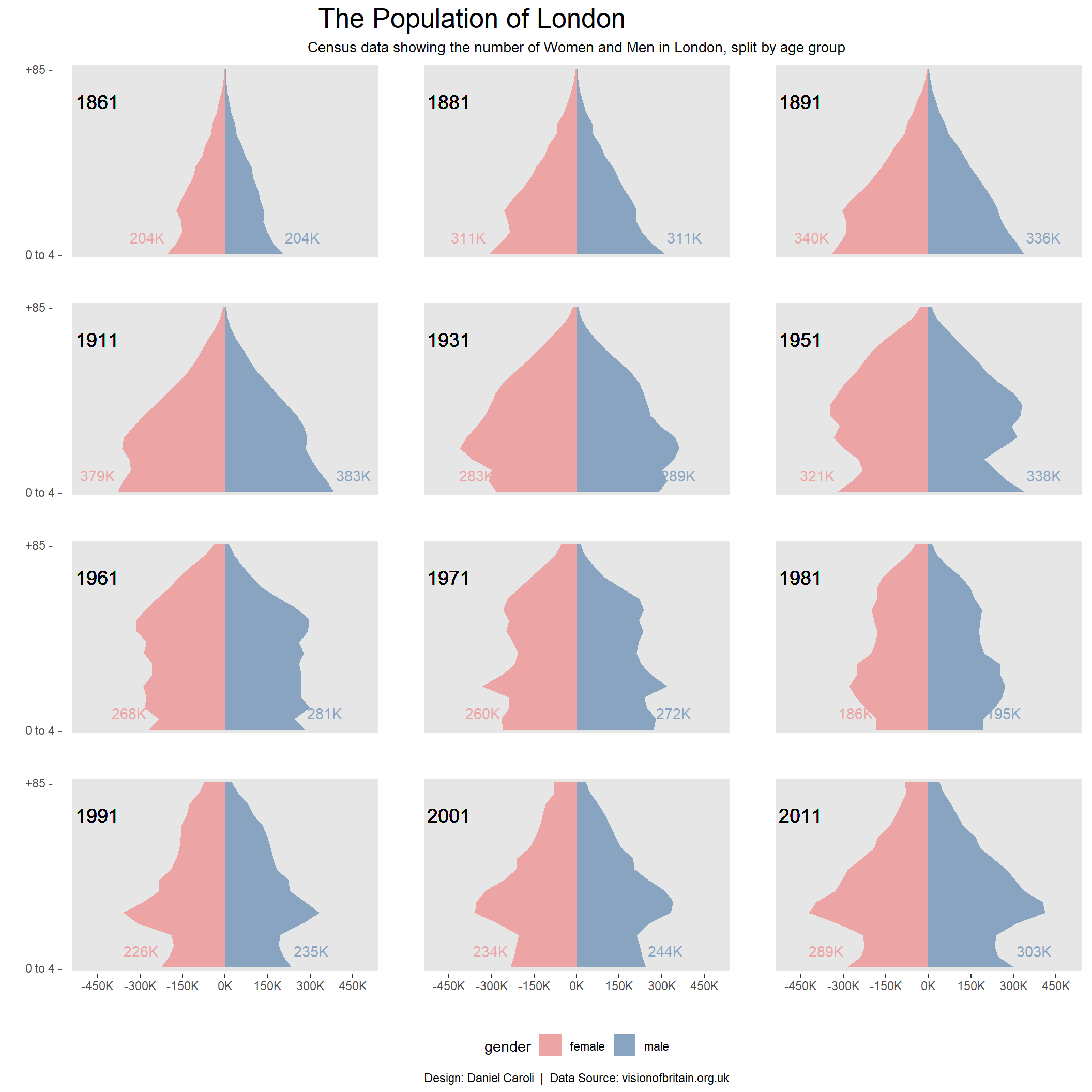
The image below was featured in Tableau Public Gallery. https://public.tableau.com/profile/daniel.caroli#!/vizhome/ThePopulationofLondon/Main

Data Preparation

Below is the accompanying code to reproduce the chart above. The data was sourced from data export options in the link above.

library(dplyr)
library(tidyr)
library(ggplot2)
library(readr)
library(janitor)

population_london <- readr::read_csv("./data/Adjusted_data.csv") %>% 
  clean_names() %>% 
  select(age_group, label_position, female, calculation1, male, year) %>% 
  mutate(
    female = gsub(pattern = "K", replacement = "", x = female) %>% as.numeric,
    female = female*1000*(-1),
    male   = gsub(pattern = "K", replacement = "", x = male) %>% as.numeric,
    male   = male*1000,
  ) %>% 
  pivot_longer(
    cols = c("female","male"),names_to = "gender", values_to = "population"
  )

population_london$age_group <- factor(
  population_london$age_group, 
  levels = unique(population_london$age_group)
)

GGPLOT2

ggplot(data = population_london) +
  geom_ribbon(aes(x = age_group, ymin = 0, ymax = population, group = gender, fill = gender)) +
  scale_fill_manual(
    values = c("#ECA5A4", "#89A4C0")
  ) +
  geom_text(x = 15, y = -450000, aes(label = year), size = 5) +
  geom_text(data = dplyr::filter(population_london, age_group=="0 to 4") %>% 
              mutate(
                population_new = ifelse(population<0,population-70000, population+70000),
                label = paste0(gsub(pattern = "(000)|(-)",replacement = "", x = population),"K")),
    aes(x = as.numeric(age_group)+1.5, y = population_new, label = label, colour = gender)
  ) +
  scale_color_manual(
    values = c("#ECA5A4", "#89A4C0")
  ) + 
  scale_x_discrete(
    labels = c("0 to 4 -",rep("",16),"+85 -")
  ) +
  scale_y_continuous(
    limits = c(-500000, 500000),
    breaks = seq(from = -450000, to = 450000, by = 150000),
    labels = paste0(seq(from = -450, to = 450, by = 150), "K")
  ) +
  coord_flip() + 
  facet_wrap(~ year, ncol = 3) +
  theme_classic() +
  labs(
    title = "The Population of London                           ",
    subtitle = "Census data showing the number of Women and Men in London, split by age group",
    caption = "Design: Daniel Caroli  |  Data Source: visionofbritain.org.uk"
  ) +
  xlab("") + ylab("") +
  theme(
    axis.ticks.y = element_blank(),
    axis.text.y = element_text(hjust = 0),
    strip.background = element_blank(),
    strip.text.x = element_blank(),
    legend.position = "bottom",
    panel.background = element_rect(fill = "#E6E6E6", colour = "NA"),
    panel.border = element_rect(colour = "white", fill=NA, size=2),
    axis.line = element_line(colour = "white"),
    panel.spacing = unit(2, "lines"),
    plot.title = element_text(size = 20, hjust = 0.5),
    plot.subtitle = element_text(size = 10.5, hjust = 0.5),
    plot.caption = element_text(hjust = 0.5)
  )